

Description of the Simulations#
The simulation process consists of the following steps:
Air shower and Cherenkov light production using the CORSIKA simulation code [3]:
Extensive air shower simulation: The interaction of a primary particle (very high-energy \(\gamma\)-ray or background cosmic ray) in the atmosphere and the development of the particle cascade through the atmosphere is simulated.
Cherenkov light production and propagation: Cherenkov photons emitted by the particles traversing the atmosphere are traced to the ground taking into account scattering and absorption in the atmosphere by molecules and aerosols. For efficiency purposes, Cherenkov photons are not simulated one by one but in bunches. Only those photons expected to fall within a fiducial sphere centered on the rotation angle of the telescopes and with a radius larger than that of the telescope dish are recorded (see Figure 1).
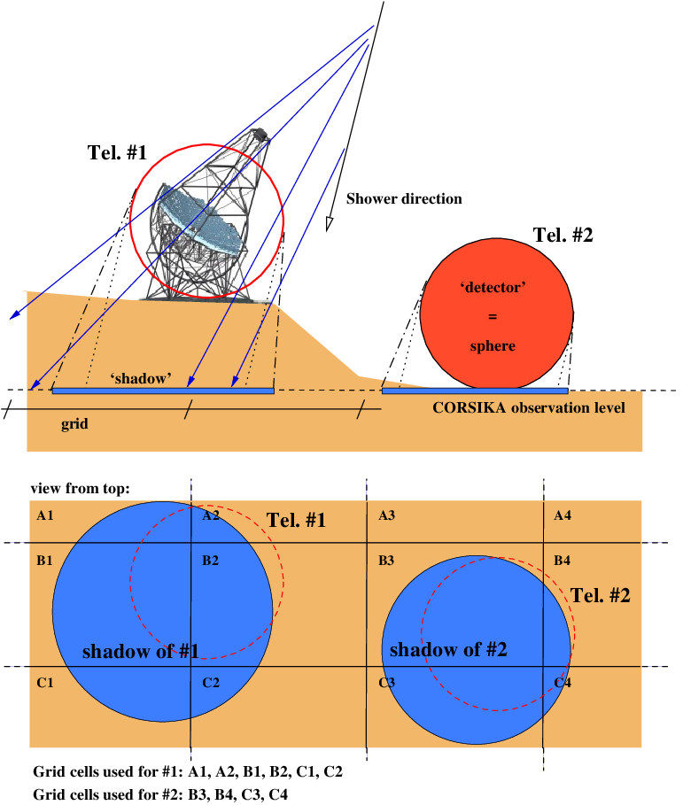
Definition of grid cells at the detection level to which a detector sphere gets linked for detailed inspection of intersections of photon bunches with the sphere. The shadow of a sphere is large enough to include all Cherenkov light emitted up to 10 degrees from the shower direction and intersecting the sphere. Figure taken from [1].#
For each event the following parameters are available at the end of this step: The type and energy of the primary particle; a list of Cherenkov photons with their position on the ground or the telescope level, wavelength, incident angle, emission height, arrival time (counted since entrance of the primary particle into the atmosphere), and the Cherenkov photon bunch size. This list of photons hitting the fiducial sphere is passed to the package [1] for a detailed simulation of the telescope.
Simulation of the detector response using the sim_telarray package [1]:
Extinction (absorption and scattering) losses of Cherenkov photons traversing the atmosphere.
Ray-tracing of the Cherenkov photons through the telescope optics (more details below).
Camera simulation, trigger, and readout (more details below). This step includes the addition of noise photons from the night-sky background.
Optics#
The propagation of Cherenkov photons through the telescope optics includes the effects of shadowing, the simulation of reflection (wavelength dependent) and scattering of photons off individual mirrors.
A precise ray-tracing of both incoming and reflected photons, taking into account the shadowing due to masts, trusses and camera lid can be performed using sim_telarray, but is not done in standard production as it requires a lot of computing time. Therefore, only the shadowing of the camera, controlled by the parameters camera_body_diameter (actual flat-to-flat distance for square and hexagonal shapes) and camera_depth, and the shadowing of the secondary mirror and its baffle (if applicable) is handled explicitly. The shape of the camera can be circular, square or hexagonal, controlled with the camera_body_shape parameter. The effect of shadowing by other elements, like the masts, is taken into account by parametrising the fraction of photons lost as a function of off-axis angle. The parameters are passed to sim_telarray through the telescope_transmission parameters set.
Reflectivity#
The mirror reflectivity is considered in the simulation as a function of the photon wavelength and (optionally) the photon incidence angle. It is passed to sim_telarray through the mirror_reflectivity parameter. If the reflectivity is given only as a function of the photon wavelength, then it should be given for the typical (average) incident angle. For dual mirror optics a different reflectivity for the secondary mirror can be specified with mirror_secondary_reflectivity. Only specular reflectivity is considered in the simulation of Cherenkov light. Total reflectivity (the combination of specular and diffuse reflection) is only required for the calculation of the night-sky background rates.
Camera plane optics#
After reflection on the primary mirror (and secondary mirror, if dual mirror optics is considered), the photon is traced to the camera focal plane. In the case of dual mirror optics, the focal plane shape of the camera is defined by a polynomial with parameters set by focal_surface_parameters. The pixel positions, grouped by modules, are then defined to exist on this surface and, if the parameter pixels_parallel is set to be true, they will also be orientated such that they are aligned with the focal plane (otherwise they are orientated perpendicular to the telescope axis). The coordinates of the pixels are defined by the projection onto the \(x\)–\(y\) plane from a curved surface. In the case of single mirror optics the camera focal plane surface is considered flat.
The wavelength dependence transmission of any window or filter in front of the camera body is taken into account (camera_filter). A two-dimensional data file may be provided to the model in order to take into account both the wavelength and photon incidence angle dependence. As a final step of the optics simulation, the angular acceptance of the pixels, as well as that of the Winston cones (if applicable), is taken into account. The shapes of pixel entrance and unobstructed photo-cathode can be hexagonal, square, or circular. The pixel positions, entrance shape, funnel shape, diameter and depth, as well as angular and wavelength acceptance tables, are given in a separate configuration file, passed to sim_telarray through the camera_config_file parameter.
Simulation of single mirror telescope optics#
The optics for a single mirror telescope are defined by the focal_length, the dish shape, and the position of the individual mirrors.
The parameters describing the individual mirrors are defined through a separate configuration file, given as input through the parameter. The list contains the position of each mirror tile (\(x_i\), \(y_i\)), perpendicular to the optical axis, together with its shape, size and individual focal length \(f_i\). The \(z_i\) positions of the mirror tiles is optional and if they are omitted, the mirrors will be positioned following variants of a shape, taking mechanical accuracies into account, defined by the parameter . Mirror tiles can have either individual focal lengths, defined with different \(f_i\) values in the table; all the same focal lengths, set with the parameter; or automatically optimized focal lengths, calculated from the desired dish shape and (\(x_i\), \(y_i\)). The optimum focal lengths of spherical tiles on a parabolic dish can be obtained by calculating the principal (maximum and minimum) radii of curvature of the paraboloid at the position of the mirror segment. Half the geometric mean, i.e. \(0.5 (r_{\text{min}} r_{\text{max}})^{1/2}\), is used for automatically optimized focal lengths, but the simple distance of the mirror tile to the system focus would be reasonable as well, as the two lead to almost the same result. Mirror tiles can be of hexagonal, square, or circular shape.
Optical PSF#
The optical PSF of the telescope is affected by
the type of optics and size of mirror tiles;
the micro-roughness of the mirror surface;
the uncertainty on the focal length of the different mirror tiles;
random misalignments and misplacements of the mirror tile on the dish.
Items 2 and 3 are intrinsic to each mirror tile and their effect can be quantified in the laboratory by e.g. 2F measurements of single mirror tile spot size. In the simulations, the small-scale roughness of the mirror surface is taken into account with a Gaussian smearing of the reflected photon direction according to an r.m.s. spread given by the parameter mirror_reflection_random_angle (for a better description of the tails of the PSF, optionally the sum of two Gaussians can be used). The uncertainty on the mirror tile focal length is considered through random fluctuations in mirror focal lengths and is controlled by the parameter random_focal_length. These two parameters should be adapted to match the measurements in the laboratory on the mirror tiles.
To take into account the effect of the variation of the alignment of the mirrors with respect to the nominal alignment, two additional sets of parameters are used to smear the horizontal and vertical directions of the reflected photons:[1] mirror_align_random_horizontal (\(\theta-0\),\(\alpha-h\), \(\beta-h\), \(\gamma-h\)) and mirror_align_random_vertical (\(\theta-0\),\(\alpha-v\), \(\beta-v\), \(\gamma-v\)) respectively. These sets of parameters take into account the zenith angle dependence of this effect into account, following any dynamical alignment performed. The spread in the horizontal direction is given by,
\(\sigma_h = \sqrt{{\alpha_h}^{2} + {\beta_h}^{2}(\sin{\theta} - \sin{\theta_0})^2 + {\gamma_h}^{2}(\cos{\theta} - \cos{\theta_0})^{2}} \, ,\)
while the spread in the vertical direction is,
\(\sigma_v = \sqrt{{\alpha_v}^{2} + {\beta_v}^{2}(\sin{\theta} - \sin{\theta_0})^2 + {\gamma_v}^{2}(\cos{\theta} - \cos{\theta_0})^{2}} \, .\)
The zenith angle at which the PSF has been measured is given by \(\theta_0\). The parameters \(\alpha_h\), \(\beta_h\), \(\gamma_h\), \(\alpha_v\), \(\beta_v\) and \(\gamma_v\) are obtained from a fit of the experimental optical PSF of the full telescope optics, taking into account the single-mirror tile point-spread function as described above. The \(\sigma_h\) and \(\sigma_v\) are used for a Gaussian randomisation of the mirror alignment.
Dual mirror telescope optics#
The size, shape and position of the primary mirror tiles are given via the primary_segmentation parameter, either as the parameters of the segments of the ring or as a list explicitly defining the parameters of each mirror in the case of hexagonal or circular mirrors.
The mirror tiles are positioned on the primary and secondary dish following shapes defined by polynomials with parameters set by primary_mirror_parameters and secondary_mirror_parameters respectively.
Optical PSF#
The optical PSF of the telescope is affected by
the type of optics and size of mirror tiles;
the micro-roughness of the mirror surface;
the shape deviation of the single mirror tiles from the polynomials defining the dual optics;
random misalignments and misplacements of the mirror tile on the dish.
Items 2 and 3 are intrinsic to each mirror tile and their effect can be quantified in the laboratory by measuring the spread of directed-light on the single mirror tiles (item 2), and by determining the difference between the expected and measured direction of reflected light (item 3). More details on these measurements can be found in Ref. [2]. In the simulations, the small-scale roughness of the mirror surface is taken into account with a Gaussian smearing of the reflected photon direction according to an r.m.s. spread given by the parameter mirror_reflection_random_angle (for a better description of the tails of the PSF, optionally the sum of two Gaussians can be used). At the moment, the effect of items 3 and 4 is not taken into account in the simulation in the case of dual mirrors. An effective way to take into account the effect of item 4 is to increase the mirror_reflection_random_angle parameter in order to match measurements made with the telescope.
Camera#
The simulation of the photon detectors takes into account collection efficiencies, amplitude fluctuations, signal shapes, after-pulsing (specific for photomultipliers), optical cross talk (specific for SiPM), and the dynamic range due to the finite number of cells per device. The camera simulation also include efficiency and gain variations between pixels. It is worth noting here that it is assumed that structural noise in the camera is calibrated out on the fly; what remains, and what is simulated here, is the cell-wise uncorrelated Gaussian noise that remains.
Quantum efficiency#
The main relevant efficiency parameter for the camera is the quantum efficiency (photon detection efficiency for SiPM) as a function of wavelength, given in table form in a file passed to sim_telarray through the parameter quantum_efficiency. The quantum efficiency can vary between the photo detectors. The magnitude of the variation is set by a wavelength-independent parameter, qe_variation. There is an option to set the photo-detector collection efficiency, pm_collection_efficiency (this is generally set to 1.0, as the non-amplified photo-electrons are included in the amplitude distribution of the single-p.e. spectrum). Average gain and gain variation of the photo detectors are set through pm_average_gain and gain_variation respectively. The pm_average_gain is only relevant for the DC current as it is checked to turn pixels with star light off.
Transit time#
The simulation includes the mean transit time through the detector (pm_transit_time) and the transit time jitter of individual photons The trigger time for the signal is calculated from the median of the photon arrival times. The time defining the signal is calculated from the median of the photo arrival times. A fixed time delay (photon_delay) can also be added. Finally, the transit time also includes a correction factor to include the quantum efficiency and voltage variation, along with variation of the FADC amplitude resulting from gain variation, such that
where the voltage relative to the expected average is
Generally, from equations above, higher than nominal voltage leads to a negative delay, while lower voltage results in positive delay. The quantity \(\zeta\) is defined as
if \({\textbf{pm_gain_index}} > 0\), and
otherwise. The value of the random relative pixel gain, \(g_{\text{rel}}\), is set as
when flatfielding is used (\(\textbf{flatfielding} = 1\)), or as
without flatfielding (\(\textbf{flatfielding} = 0\)). The signal amplitude scales (\(\textbf{fadc_amplitude}\), \(\textbf{discriminator_amplitude}\), and \(\textbf{adjust_gain}\)) are set separately, but they are all scaled by the same \(g_{\text{rel}}\).
The parameter \(\textbf{transit_time_compensate}\) should be set in case transit time differences are compensated by programmable delays. The compensation itself is done in nanosecond steps set by \(\textbf{transit_time_compensate_step}\) with an assumed accuracy in its evaluation of \(\textbf{transit_time_compensate_error}\). With TRANSIT defined as the per-channel delay, the compensation is applied as follows:
For a very simple illustration of the Discriminator signal creation, see Figure 2.
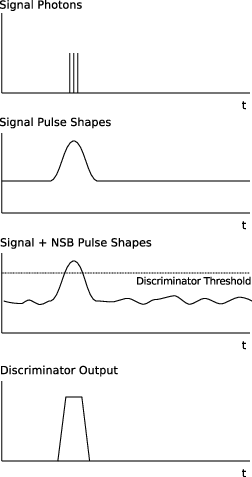
Very simple illustration of the Discriminator signal creation.#
Photo-detector response#
The single photo-electron amplitude is randomly drawn from the response spectrum set by \(\textbf{single_pe_spectrum}\). The same is done for the night-sky background (NSB) photons, however these are sampled from the single photo-electron spectrum which includes after-pulsing. The amount of NSB in each pixel is set by \(\textbf{nsb_rate}\) multiplied by \(\textbf{pixel_area}\) and then drawn from a Poisson distribution around this value.
Once it has been determined whether or not the photons were detected, the simulation of the electronics begins (trigger and readout). The electronics in sim_telarray are described by way of a comparator/discriminator for the trigger and an FADC for the readout.
Trigger#
Three different trigger logics are available in the simulations, analog and digital sum, and a majority trigger logic (selected with default_trigger).
The input signal sent to the discriminator is calculated from the list of photoelectrons, each assigned an amplitude defined by the parameter discriminator_amplitude, scaled to include the gain variation (gain_variation) and quantum efficiency variations qe_variation,
The shape of each pulse signal is generated from the input discriminator pulse shape file (discriminator_pulse_shape) and added to the total discriminator signal, shifted by the appropriate time. The input signal to the discriminator is oversampled with respect to the FADC sampling. Typically, the sampling rate in the simulation of discriminator input signals is four times higher than the FADC sampling rate (fadc_mhz). The discriminator logic is applied to the resulting waveform.
Camera trigger logic - AnalogSum#
The simulation of the trigger logic for the analog sum trigger is defined as follows:
An (optional) shaping of the input signal is applied using a shaper signal defined in \(\textbf{analog_shaper_signal}\).
An (optional) time offset, \(\textbf{analog_time_offset}\), used in the convoluted signal of the “discriminator input” signal \(\times\) the \(\textbf{analog_shaper_signal}\) (effectively a convolution kernel).
If necessary, the analog signal in each pixel is clipped (clipping threshold defined by \(\textbf{analog_clipping_threshold}\)).
The analog signals from clusters of adjacent trigger modules are summed. The clusters and modules are defined in the \(\textbf{trigger_module_config}\). A trigger module is composed of seven pixels and a trigger cluster consists of three modules, 21 pixels in total. One module can be part of a few trigger clusters, such that the clusters overlap.
The trigger fires if the sum over all pixels in a trigger cluster is higher than a predefined value, \(\textbf{analog_trigger_threshold}\).
Camera trigger logic - DigitalSum#
The simulation of the trigger logic for the digital sum trigger is defined as follows:
An (optional) shaping of the input signal is applied using a shaper signal defined in dsum_shaping_file.
An (optional) time offset in FADC bins, (dsum_offset), used in the convoluted signal of the ``discriminator input’’ signal \(\times\) the dsum_shaping_file (effectively a convolution kernel).
If necessary, the digital signal in each pixel can be clipped either before or after shaping. The clipping thresholds are defined respectively by dsum_pre_clipping and dsum_clipping.
The digital trigger logic, defined in the camera_config_file, is then applied and can be either of the following options:
The digital signals in trigger clusters of adjacent pixel patches are summed and the trigger fires if the sum over all pixels in a cluster is higher than a predefined value, dsum_threshold. A patch is composed of three adjacent pixels and a trigger cluster consists of three patches, nine pixels in total. One patch can be part of a few trigger clusters, such that the clusters overlap. % FIXME See figure when plot is ready. An example for this case for the definition in the camera_config_file is ``DigitalSumTrigger * of 1719[1724,1726] 1716[1717,1718] 1732[1733,1734].”
SmartPixel logic: e.g. a pixel cluster of seven pixel clusters where the central pixel must have fired (would be a line in the camera_config_file like ``Trigger * of 561 562 597 +598 599 633 634’’, with the smart pixel indicated by the ‘+’).
Camera trigger logic - Majority#
The simulation of the majority trigger logic is defined as follows:
The discriminator input signal from each pixel (or sum of multiple pixels in the case of super pixels) is compared to the \(\textbf{majority_discriminator_threshold}\), taking into account channel-to-channel variations \(\textbf{channel_variation}\).
The time and signal sum above the thresholds are calculated and compared to values defined by the parameters \(\textbf{majority_time_threshold}\) and \(\textbf{majority_signal_threshold}\), taking into account the corresponding channel-to-channel variations for these parameters.
The signal at the output of the discriminator is generated based on the following parameters: \(\textbf{majority_output_signal}\), \(\textbf{majority_output_time}\), \(\textbf{majority_output_amplitude}\), and \(\textbf{majority_output_shape}\).
The majority logic, defined in the \(\textbf{majority_trigger_config}\), is then applied and can be either of the following options:
SmartPixel logic: e.g. a pixel cluster of 7 pixels where the central pixel must have fired (would be a line in the \(\textbf{majority_trigger_config}\) like “Trigger * of 561 562 597 +598 599 633 634”, with the smart pixel indicated by the ‘+’).
A majority trigger of a number of pixels (or super pixels) inside a group of pixels (or super pixels). The list of pixels composing the super pixel and the trigger group must be defined explicitly in the camera config file, e.g., “MajorityTrigger * of 0[1,32,33] 64[65,96,97] 2[3,34,35] 66[67,98,99]”, where 0[1,32,33] indicates one of the super pixels and 0, 64, 2 and 66 indicate the pixel group. A * for the number of pixels required for a trigger means that it will be replaced by the per-telescope default, configured with the parameter \(\textbf{majority_default_threshold}\).
A minimum time or signal sum over threshold for each sector is required for a trigger, with the thresholds defined by \(\textbf{sector_time_threshold}\) and \(\textbf{sector_signal_threshold}\) respectively.
an optional current limit can be applied with \(\textbf{current_limit}\), excluding any pixels from the trigger if they exceed a certain current, calculated as,
The $\textbf{current_limit}$ used for the DC current is the same as
used for the single-p.e. amplitudes (while that part in gain
differences resulting from QE differences, compensated through HV
adjustment for uniform flatfield, cancels out here). The parameter
$\textbf{current_limit}$ also applies for the discriminator input signal and all FADC
channels (and also the per-pixel random value resulting from $\textbf{pixel_random_value}$).
For a single telescope trigger, a minimum number of super pixels is required, \(\textbf{min_super_pixels}\), based on a coincidence of the discriminator outputs.
Readout#
The FADC signal is treated in a similar fashion as the discriminator signal, with the amplitude set by fadc_amplitude (scaled with the quantum efficiency and gain_variation, similarly to the discriminator amplitude),
The FADC pulse shape is set by a table passed to sim_telarray through the fadc_pulse_shape parameter. The number of bins to be simulated for the FADC signal is set by the parameter fadc_bins. The number of readout bins is defined by fadc_sum_bins, starting fadc_sum_offset before the actual trigger (Note that the number of simulated bins needs to be large enough to allow the readout bins to shift in order to keep the trigger in the same time bin, this will be obvious in events with a large time gradient). The maximum signal level in an FADC channel can be set with fadc_max_signal or fadc_max_sum.
Each time bin is assigned a pedestal value defined by the parameter fadc_pedestal. The optional channel-to-channel variation is set with fadc_var_pedestal (random Gaussian). Along with the pedestal, Gaussian noise set with fadc_noise is added in the digitization process to each bin (note once again that there is no implementation of structured noise within the camera). For a very simple illustration of the FADC signal creation, see Figure 3.
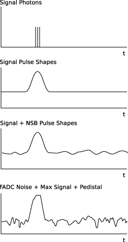
Very simple illustration of the FADC signal creation.#
Derived MC parameters#
The following parameters are derived from dedicated simulations runs in combination with several parameters of the MC Model:
night_sky_background
The photo-electron rate per pixel due to night-sky background is calculated using the nominal NSB rate and spectrum (see CTA glossary on Jama), taking into account the mirror area, reflectivity, shadowing, camera window transmission, light guides, and photo-detection efficiency. See \(\textbf{night_sky_background}\) for the value obtained for \(\textbf{nsb_rate}\).
trigger_threshold
The trigger threshold is derived from MC simulations using the safe threshold definition, which is applied in a similar way to all CTA telescope types. The safe threshold is defined as the intersection point of the trigger rate curve for night-sky background (at \(2\times\) dark conditions) and \(1.5\times\) the trigger rate from cosmic-ray protons. For the reference spectra for NSB and cosmic-ray protons, see the CTA Glossary on the Jama system (NSB definition; reference proton flux).
Bibliography#
Konrad Bernlohr. Simulation of Imaging Atmospheric Cherenkov Telescopes with CORSIKA and sim_telarray. Astropart. Phys., 30:149–158, 2008. arXiv:0808.2253, doi:10.1016/j.astropartphys.2008.07.009.
Konrad Bernlohr and Nepomuk Otte. Test measurements to validate and improve the monte carlo models of cta telescopes. https://gitlab.cta-observatory.org/cta-consortium/aswg/simulations/documents/mc-measurements/-/blob/master/mcmeas.pdf.
D. Heck, G. Schatz, T. Thouw, J. Knapp, and J. N. Capdevielle. CORSIKA: A Monte Carlo code to simulate extensive air showers. Forschungszentrum Karlsruhe Report FZKA-6019, 1998.